Chapter 9 Decision Tree (W9)
9.1 What is a Decision Tree?
What is a Decision Tree?: 의사결정나무는 무엇인가?
어느 대안이 선택될 것인가라는 것과 일어날 수 있는 불확실한 상황 중에서 어떤 것이 실현되는가라는 것에 의해 여러 결과가 생긴다는 상황을 나뭇가지와 같은 모양으로 도식화한 것이다. 의사결정 나무를 구성하는 요소에는 결정나무의 골격이 되는 대안과 불확실한 상황, 결과로서의 이익 또는 손실, 불확실한 상황과 결과가 생기는 확률이 있다. 이들의 요소가 결정점과 불확실점으로 결합되어 의사결정나무를 만들게 된다. (HRD 용어사전)
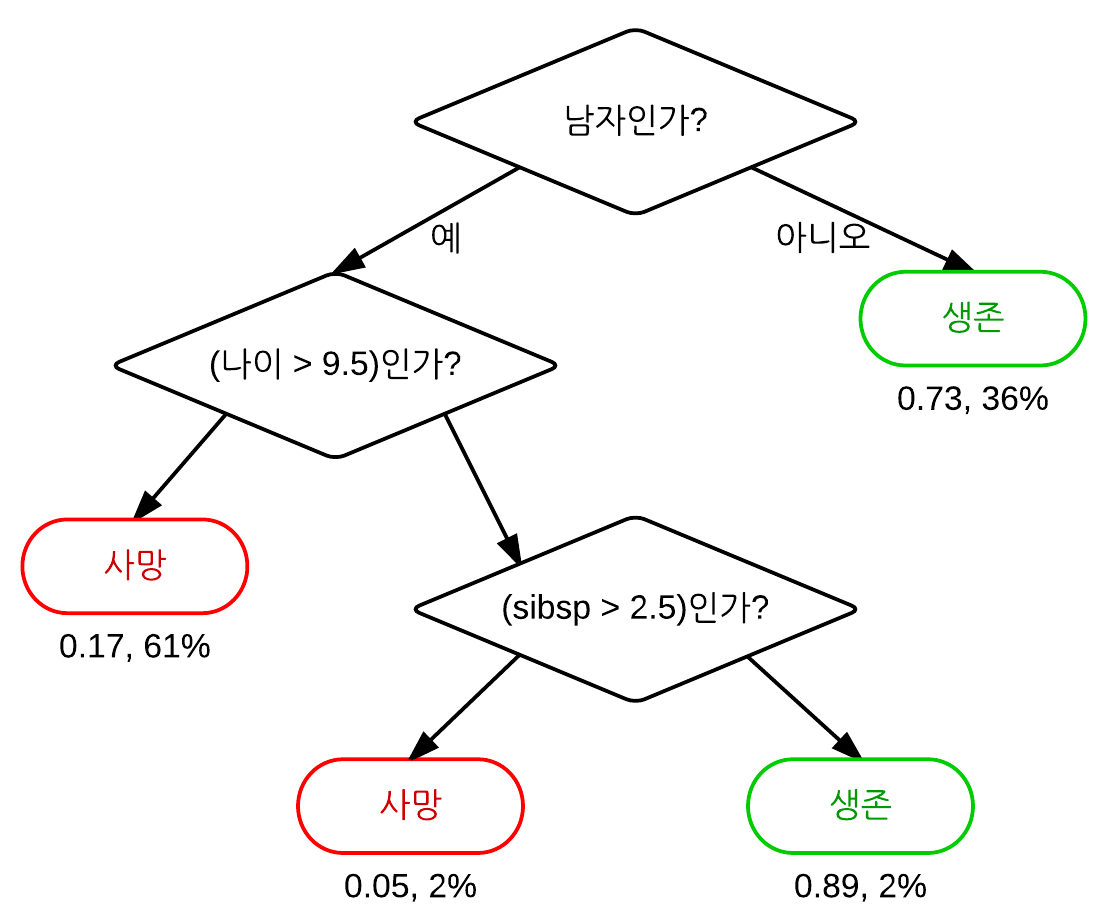
Figure 9.1: 타이타닉 생존자
https://ko.wikipedia.org/wiki/%EA%B2%B0%EC%A0%95_%ED%8A%B8%EB%A6%AC_%ED%95%99%EC%8A%B5%EB%B2%95
- 의사결정나무와 관련된 r패키지는 크게 3가지가 있으며, party 패키지를 이용한 분석을 해보자.
- tree
- rpart
- party
- 훈련데이터 vs. 테스트데이터 비율로 나누기 위해 caret 패키지 사용
- Training (70%): Test(30%)
data(iris)  # iris dataset
str(iris)  # check iris dataset
## 'data.frame': 150 obs. of 5 variables:
## $ Sepal.Length: num 5.1 4.9 4.7 4.6 5 5.4 4.6 5 4.4 4.9 ...
## $ Sepal.Width : num 3.5 3 3.2 3.1 3.6 3.9 3.4 3.4 2.9 3.1 ...
## $ Petal.Length: num 1.4 1.4 1.3 1.5 1.4 1.7 1.4 1.5 1.4 1.5 ...
## $ Petal.Width : num 0.2 0.2 0.2 0.2 0.2 0.4 0.3 0.2 0.2 0.1 ...
## $ Species : Factor w/ 3 levels "setosa","versicolor",..: 1 1 1 1 1 1 1 1 1 1 ...head(iris) # read first 6 rows## Sepal.Length Sepal.Width Petal.Length Petal.Width Species
## 1 5.1 3.5 1.4 0.2 setosa
## 2 4.9 3.0 1.4 0.2 setosa
## 3 4.7 3.2 1.3 0.2 setosa
## 4 4.6 3.1 1.5 0.2 setosa
## 5 5.0 3.6 1.4 0.2 setosa
## 6 5.4 3.9 1.7 0.4 setosalibrary(caret) # seperate data (training: test)## Loading required package: latticeset.seed(1000) #reproducability setting
intrain <- createDataPartition(y = iris$Species, p = 0.7, list = FALSE)
train <- iris[intrain, ]
test <- iris[-intrain, ]party 패키지를 사용하는 방법
library(party)## Loading required package: grid## Loading required package: mvtnorm## Loading required package: modeltools## Loading required package: stats4## Loading required package: strucchange## Loading required package: zoo##
## Attaching package: 'zoo'## The following objects are masked from 'package:base':
##
## as.Date, as.Date.numeric## Loading required package: sandwichMyDecisionTree <- ctree(Species ~ Sepal.Length + Sepal.Width +
Petal.Length + Petal.Width, data = train)
plot(MyDecisionTree)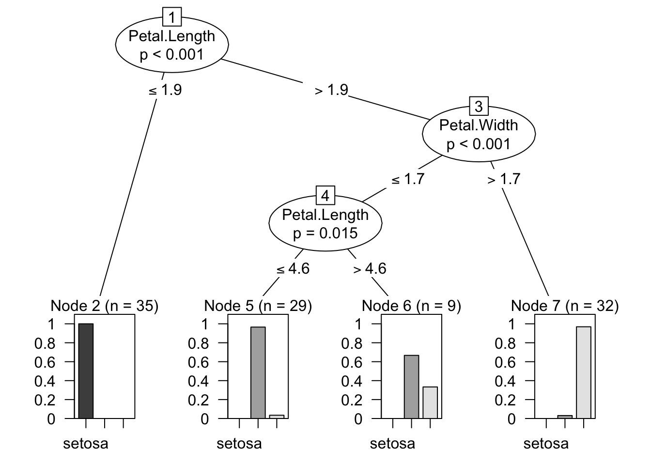
MyPrediction <- predict(MyDecisionTree, test)  # test dataset으로 확인해보자
confusionMatrix(MyPrediction, test$Species)
## Confusion Matrix and Statistics
##
## Reference
## Prediction setosa versicolor virginica
## setosa 15 0 0
## versicolor 0 15 1
## virginica 0 0 14
##
## Overall Statistics
##
## Accuracy : 0.9778
## 95% CI : (0.8823, 0.9994)
## No Information Rate : 0.3333
## P-Value [Acc > NIR] : < 2.2e-16
##
## Kappa : 0.9667
## Mcnemar's Test P-Value : NA
##
## Statistics by Class:
##
## Class: setosa Class: versicolor Class: virginica
## Sensitivity 1.0000 1.0000 0.9333
## Specificity 1.0000 0.9667 1.0000
## Pos Pred Value 1.0000 0.9375 1.0000
## Neg Pred Value 1.0000 1.0000 0.9677
## Prevalence 0.3333 0.3333 0.3333
## Detection Rate 0.3333 0.3333 0.3111
## Detection Prevalence 0.3333 0.3556 0.3111
## Balanced Accuracy 1.0000 0.9833 0.9667- 정확도 (Accuracy): 97.78%
- No Information Rate: 데이타가 임의적으로 있을 경우의 정확도
- 그러므로 정확도가 No Information Rate보다 높아야 예측이 잘되는 것 (97.78% > 33.33%)